Trees: Prufer code

The goal of this section is to prove Cayley’s theorem:

Theorem (Cayley):

There are $n^{n-2}$ trees on $n$ labelled vertices.

For instance, if there are three vertices, then there’s only one tree up to isomorphism: the path of length 2. There are apriori 3!=6 ways to label the vertices of this tree, but since there’s an isomorphism from the tree to itself that keeps that the middle vertex fixed but switches the two end vertices, we’re really counting each of these labels twice, and we find out that there are really 3 different labelled trees on 3 vertices.

This theorem is in the algorithms section because we will prove it by constructing the Prufer code, giving a bijection between labelled trees, and n-2 tuples of numbers between 1 and n. But first we will need to establish a few basic facts about trees, that will be useful elsewhere.

Leafs

A useful concept when studying trees is that of a leaf:

Definition

A leaf in a tree is a vertex of degree 1.

Lemma

Every finite tree with at least two vertices has at least two leaves.

Proof 1: using paths

Suppose $T$ is at tree. Since $T$ has at least two vertices, at has at least one edge. Pick any edge $e$, say, between $a$ and $b$. If the vertex $a$ is a leaf, we have at least one leaf. If not, there is another edge incident to $a$. and we can start a path from $a$ away from $e$ following this edge. As long as the end vertex of our path is not a leaf we may continue our path, and we will never return to a vertex we have already encountered, since trees have unique paths between vertices. Since $T$ is finite, the path must eventually terminate – i.e., find a leaf.

Following the same argument from the vertex $b$ produces another leaf. $\square$

Proof 2: using handshaking

We will use that $\Gamma$ is connected, has $n>2$ vertices, and $n-1$ edges.

Since $\Gamma$ is a tree it is connected; since it has connected and has two vertices it cannot have any vertices of degree 0.

Thus, if we assume for a contradiction that $\Gamma$ has no leaves, then every vertex $\Gamma$ had degree at least two. Since we know $\Gamma$ has $n$ vertices and $n-1$ leaves, applying the handshaking lemma gives:

$2n-2=2 |E(\Gamma)|=\sum_{v\in V(\Gamma)} d(v)\geq \sum_{v\in V(\Gamma)} 2=2n$ a contradiction. For the inequality to hold, $\Gamma$ must have at least two vertices of degree 1. $\square$

Leaves will play a very important role in this afternoon’s lecture on the Prüfer code. In the meantime, we point out that the handshaking argument we give another application of the handshaking lemma argument above. Recall that in the last lecture we stated the following, but did not provide a full proof:

Proposition

Let $\Gamma$ be a graph with $n$ vertices. The following are equivalent:

1. $\Gamma$ is a tree.
2. Between any two vertices $a,b\in V(\Gamma)$, there is a unique path.
3. $\Gamma$ is connected, but removing any edge makes $\Gamma$ disconnected.
4. $\Gamma$ has no cycles, but adding any edges to $\Gamma$ creates a cycle.
5. $\Gamma$ is connected and has $n-1$ edges
6. $\Gamma$ has no cycles and has $n-1$ edges

Trying to show all of these are equivalent takes a bit of time and is a slightly annoying; but we’re going to want the fact that a connected graph $\Gamma$ with $n$ vertices is a tree if and only if it has $n-1$ edges.

Lemma

$\Gamma$ is a tree if and only if it has $n$ vertices and $n-1$ edges.

Proof

We will use induction for both directions. As a base case, the result is clear if $n$ is 1 or 2. Thus, we assume that the theorem holds for all connected graphs with $k<n$ vertices, and we must show that it holds for graphs with $n$ edges.

Suppose we know $\Gamma$ is a tree, and we want to prove it has $n-1$ edges. By the above lemmas, we know $\Gamma$ has a leaf, and deleting that vertex and the edge next to it we get a smaller tree $\Gamma^\prime$ with $n-1$ vertices. By induction, the theorem holds for $\Gamma^\prime$, and so it has $n-2$ edges; adding $e$ back, we see that $\Gamma$ had $n-1$ edges as desired.

For the other direction, suppose we know that $\Gamma$ is connected and has $n-1$ edges, but don’t know that $\Gamma$ is a tree. We still know that $\Gamma$ has at least two vertices of degree 1, as the handshaking lemma argument given above only uses the facts that $\Gamma$ is connected and has the right number of leaves.

But then we can delete one of the vertices of degree 1 and the edge next to it and preceed as above; the resulting graph $\Gamma^\prime$ will be connected, have $n-1$ vertices and $n-2$ edges. Thus, by the inductive hypothesis, $\Gamma^\prime$ is a tree, and so $\Gamma$ is as well.

Chemistry Application: Alkanes

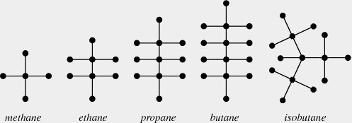
In organic chemistry, an alkane is a molecule with formula $C_nH_{2n+2}$. The simplest Alkanes are methane $CH_4$, ethane $C_2H_6$ and propane $C_3H_8$.

It appears from the graph that Alkanes are all trees; we prove that now.

Lemma

Any alkane $C_nH_{2n+2}$ is a tree.

Proof

We will use that a connected graphs on $m$ vertices with $m-1$ edges is a tree.

Any graph of a molecule is necessarily connected, and so to prove an Alkane is a tree we must count the number of vertices and edges.

There are $n+(2n+2)=3n+2$ vertices.

We count the edges using the Handshaking lemma. Carbon atoms have valency 4, and there are $n$ of them, while Hydrogen atoms have valency 1. Thus, the sum of all the degrees of the vertices is $6n+2$. The number of edges is half of these, namely $3n+1$, which is 1 less than the number of vertices. Since to be an atom it must be connected, we see that any Alkane is a tree. $\square$

Isomers

Definition

Two molecules are isomers if they have the same molecular formula, but the molecules are put together in a different way.

When there are 1, 2 or 3 carbon molecules, the only possible Alkanes is a line of carbon molecules. The resulting chemicals are methane, ethane, and propane. when $n=4$, there are two possible alignments of the Carbon atoms: in a line, which is butane, or in a `T’ shape, which is isobutane; when $n=5$, there are three different possibilities.

Around 1875, Hamilton used graph theory to count the number of isomers of the Alkane $C_nH_{2n+2}$. One can forget about the placement of the hydrogen molecules, and just count the struture of the carbon molecules; these two will be a tree. Since the valency of Carbon is four the maximum degree of a vertex in these trees will be 4, and so counting isomers of $C_nH_{2n+2}$ is equivalent to counting isomorphism classes of trees with $n$ vertices, all of degree at most 4.

Prufer Code

In this lecture, we will prove Cayley’s formula, using the Prüfer code. In particular, we will give a map $PC$ that takes in a labelled tree with $n$ vertices, and returns a string of $n-2$ numbers, each between $1$ and $n$, and an inverse map $\mathbf{Tree}$ that takes in a string of numbers and returns a labelled tree.

The starting observation is that to write down a labelled tree is the same as writing down its $n-1$ edges. Since the vertices are ordered, each edge can be written down by a pair of numbers in $\{1,\dots,n \}$. The Prüfer code begins by writing down these edges in a clever ordering.

The Prüfer code

We are now ready to introduce the Prüfer code. We begin by writing down the edges of $T$. The two vertices of each edge will be written down in a column, with the parent vertex in the top row and the child vertex on the bottom row. We record the edges in the following specific order.

First, find the lowest numbered leaf, and record its number in the bottom row. Above it, write down the number of the vertex this leaf is adjacent to, which we call the parent vertex. Now, delete that lowest numbered leaf and the edge connecting it to the rest of the tree. Find the lowest leaf on the resulting vertex, and record its number, and the number of its parent, in the next column.

Iterate this procedure until we have written down all $n-1$ edges of our tree, with the leaf numbers in the top row, and the parent numbers in the bottom row.

The list of the first $n-2$ parent numbers (i.e., all but the last), is the Prüfer code of $T$.

Example

We illustrate the construction of the Prüfer code by finding the code for the following labelled tree:

The lowest leaf is 3, which is attached to 1, so the first column goes

Thus, the Prüfer code for the above tree is 16622.

Reconstructing a tree from its Prüfer Code

It is clear from the above definition that the Prüfer code is a list of $n-2$ numbers between 1 and $n$; it is not clear that any such list of numbers is obtained, nor that any two trees give us a different set of numbers. To see this, we describe an inverse algorithm, that constructs a tree on $n$ vertices from a Prüfer code.

More explicitly, the inverse algorithm will take as input a Prüfer code, and from that Prüfer code it will reconstruct the full ordered table of edges we constructed in the Prüfer code algorithm. It should be clear from the description that the algorithm actually reproduces this table, and not some other table, and hence that the two algorithms are inverse to each other. This shows that the Prüfer code is a bijection, which proves Cayley’s formula, as there are $n^{n-2}$ valid Prüfer codes on $n$ vertices.

This algorith proceeds by figuring out the corresponding child nodes one by one. Recall that any number in our list appeared as a parent node, and so is not a leaf. At the first step, we deleted the smallest leaf. So the first child node is the smallest number that does not appear on our list.

After we recorded that edge, we deleted it; thus, the second child number is the smallest number that we haven’t

1. already used as a leaf number
2. doesn’t appear at or after the current spot as a parent.

Example

We first reconstruct the tree we did in the first example, from its code. Recall, the Prüfer code was 1 6 6 2 2.

The lowest unused number is 3, so that is the first child.

To find the next unused number, we move to the second column. 1 only appears in the first column, and so it is now the lowest number that doesn’t appear, and so it goes underneath the first 6. Moving to the third column, we have already used 1 and 3 as child nodes. The number 2 is still to appear as a parent, and so can’t be a leaf yet, and so 4 is the first number that we haven’t used yet. Similar reasoning gives 5 and 7 for the 4th and 5th column.

Finally, the last remaining edge connects the two nodes we have not used as leaves yet; in this case 2 and 6.

Spanning trees

Definition

Let $\Gamma$ be a graph. A spanning tree of $\Gamma$ is a subgraph $T\subset \Gamma$ such that $T$ is a tree and $T$ contains every vertex of $\Gamma$.

Spanning trees are useful because they are a minimal connected subgraph that lets us get to all of $\Gamma$. For instance, if the vertices are cities and the edges are roads, a spanning tree is a minimal set of edges that guarantee that you can get from any one city to another.

Examples:

• The cycle graph $C_n$ has $n$ spanning trees obtained by deleting any one edge.

• A spanning tree of the complete graph $K_n$ is the same thing as a labelled tree, so there are $n^{n-2}$ such spanning trees by Cayley’s theorem.

Lemma:

Every connected graph $\Gamma$ has a spanning tree.

Proof

By our characterisation of trees, if $T$ is connected and has no cycles, then $T$ is a tree. So it is enough to find a connected subgraph $T$ of $\Gamma$ that contains every vertex.

Let $H$ be any subgraph of $\Gamma$ that is connected and contains all the vertices of $\Gamma$. If $H$ has a cycle, we can pick any edge $e$ of that cycle and delete it, and $H$ will still be connected: any path that used $e$ can use the rest of the cycle instead.

Thus, starting from $\Gamma$, we may repeatedly remove edges from cycles and not disconnect $\Gamma$ until there are no more cycles left; the result will be a spanning tree. $\square$

Introduction to optimisation problems

One motivation for introducing trees was as the “cheapest” way of connecting $n$ points. Here, “cheapest” just means the least number of edges. In real world applications, not all edges are created equal. For example, consider the case where the vertices of $\Gamma$ represent cities, and the edges are roads connecting them. If we’re looking for the shortest path between two cities, we do not just want the least number of edges, as some roads will be longer than others, or be busy and take longer to drive. These subtleties can be addressed with a weighted graph.

Definition

A weighted graph is a graph $\Gamma$, together with a non-negative real number $w(e)$ for each edge $e\in E(\Gamma)$.

Example

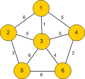
Typically, weighted graphs are presented by drawing labelling each edge of the graph with its weight:

Real world examples of weights

Even in the case where the vertices of $\Gamma$ are cities and the edges are conenctions between them, there are many possible interpretations of edges weights:

• The edge weights $w(e)$ might represent the cost of building or maintaining the road between the city
• The edge weights migth represent the distance between the cities
• The edge weights might represent travel times between the cities
• the edge weights might represent the cost of a train/plane ticket between the cities

In the next few class lectures, we will discuss the following optimisation problems for weighted graphs:

• The minimal spanning tree – finding a spanning tree $T$ of $\Gamma$ where the total cost of the edges in $T$ is the cheapest among all spanning trees of $\Gamma$.
• The shortest path – finding a path between two vertices of $\Gamma$, where the total weight of all the edges in the path is minimal among all paths between the two vertices.
• The traveling salesman problem – finding a hamiltonian cycle in a graph $\Gamma$ where the total weight of all the edges is minimal.

We will present two algorithms for finding the cheapest spanning trees. Both are “greedy algorithms”, which in some sense plan ahe

Kruskal’s and Prim’s algorithm

We now present Kruskal’s and Prim’s algorithm, both of which solve the problem of finding a minimal weight spanning tree in a weighted graph $\Gamma$. Before discussing the algorithn, let’s look at a toy example to get an idea of the problem.

Example

Consider the following weighted graph:

Obviously, there are three spanning trees, obtained by removing one of the three edges. The spanning tree A-B-C has weight 7, B-C-A has weight 6, C-A-B has weight 5, and so we have found the cheapest spanning tree.

Any finite graph will only have finitely many spanning trees, and so it is always possible to exhaustively find all of them, compute their weights, and hence find the cheapest. However, for large graphs there will be many spanning trees. For example, a spanning tree of the complete graph $K_n$ is equivalent to a labelled tree on $n$ vertices, and by Cayley we know there are $n^{n-2}$ of these trees, which grows faster than exponential or factorial! Thus, in practice, to find a minimal spanning tree we need a more efficient algorithm than brute forst checking all the possibilities.

Kruskal’s algorthm

For finding spanning trees, it turns out there are several easy algorithms that will always find the cheapest spanning tree. Many of them are greedy algorithms, which do not “plan ahead”, but rather blindly do the best possible next step. Kruskal’s algorithm is an example of these, which builds a spanning tree $T$ step by step, starting from the subgraph of $\Gamma$ consisting just of the vertices of $\Gamma$ and no edges:

1. Find the cheapest edge $e$ remaining from $\Gamma$, and remove it from $\Gamma$.
2. If adding $e$ to $T$ will not make any loops, add it to $T$. Otherwise, discard it.
3. Iterate the first two steps until $T$ is a spanning tree.

In class we now ran an example of Kruskal’s algorithm – we’ll skip that in the note, but there are many such examples available online, for instance, in this short Youtube video .

Note that to have a spanning tree, the graph $\Gamma$ must be connected. Running Kruskal’s algorithm on a disconnected graph will produce a spanning tree for each component of $\Gamma$.

Prim’s Algorithm

A different greedy algorithm to find the minimal weight spanning tree is Prim’s algorithm. Rather than always taking the cheapest edge anywhere on the graph, Prim’s algorithm starts at some vertex $v$ and builds out. At a given point it has built a tree $T$ containing the vertex $v$; call the vertices in this tree the “discovered” vertices. $T$ is initially to be just the vertex $v$, and no edges, and then the algorithm runs by repeatedly finding the cheapest edge $e$ edge that has one vertex in $T$ and one vertex not in $T$ and adding that edge (and hence a new vertex) to $T$.

Comments on minimal spanning trees

1. Although Kruskal’s algorithm only finds a single minimal spanning tree, the only time Kruskal’s algorithm has any choice is in what order to add edges with the same weight. Thus, it is possible to find all minimal spanning trees by analyzing what happens when we had a choice of edges to add.
2. There are many other algorithms that find the minimal spanning tree: for instance, the Reverse-delete algorithm is the opposite of the greedy algorithm. Rather than adding the cheapest edge possible, the Reverse-delete algorithm worries about getting “stuck” having to add an expensive edge. It continually finds the most expensive edge. If removing that edge does not disconnect the graph, it does so. If it does disconnect the graph, it keeps that edge as part of the spanning tree, and finds the next most expensive edge.

Traveling Salesman Problem

The Traveling Salesman Problem, abbreviated TSP, is the following: given a weighted graph $\Gamma$, find the cheapest Hamiltonian path; that is, the cheapest closed walk on $\Gamma$ that visits every vertex exactly once.

We begin with some basic observations:

• It is enough to consider the complete graph $K_n$. If we are given some other weighted graph $\Gamma$, we can add all the edges not in $\Gamma$ but make their weights much larger than any of the weights inside $\Gamma$.

• The problem of determining whether a given graph $\Gamma$ has a Hamiltonian cycle is a special case of the traveling salesman problem. To see this, suppose we’re given a graph $\Gamma$, and we want to determine whether it is Hamiltonian. We create a weighted $K_n$, with vertices the vertices of $\Gamma$ by giving the edge $v-w$ a very small weight $\epsilon$ if $v$ and $w$ are adjacent in $\Gamma$, and a very large weight $M$ if $v$ and $w$ are not adjacent in $\Gamma$. Then, any Hamiltonian path in $\Gamma$ would have cost $n\epsilon$, where as any path that uses an edge not in $\Gamma$ costs more than $M$. So, if we make $M>n\epsilon$, the TSP for our weighted $K_n$ will have a solution with cost less than $M$ if and only if $\Gamma$ had a Hamiltonian cycle.

Since determining whether a graph $\Gamma$ is Hamiltonian is difficult (NP complete), the TSP will also be. As such, we will not discuss any algorithms for actually solving TSP. Instead, we will discuss methods for giving upper and lower bounds for the TSP.

Upper bounds for TSP

Since the TSP asks for the cheapeast Hamiltonian cycle, taking any Hamiltonian cycle and calculating its cost will be an upper bound for the TSP. Just choosing a random Hamiltonian cycle will in general be very expensive and silly – for instance, going from Sheffield to London to Rotherham to Edinburgh to Chesterfield to Glasgow to Nottingham to Brighton is clearly not optimal.

A greedy algorithm will give a heuristically better result: we call it the nearst neighbor algorithm. At each step, simply go to the nearest city you have not already visited. This will give good results at the beginning, but since we do not do any planning ahead, it will in general give bad results, as the following example illustrates:

Consider running the Nearest Neighbor algorithm starting at $v_0$. At the first step, we have a choice – we could go to $v_1$ or to $v_9$. Suppose we go to $v_1$. After that, our choice is forced – $v_1-v_2-v_3-v_4-v_5-v_6-v_7-v_8-v_9$ costs one at each step. Now, we still have to visit $T$ before returning to $V_0$, which will cost us 10 to detour through. We clearly should have planned ahead and visited $T$ in between vertices $v_4$ and $v_5$ at a cost of 4.

The nearest neighbour algorithm for finding upper bounds is demonstrated in this video.

Clearly the nearest neighbour algorithm is not very good, and better algorithms are possible; we present it first to give a quick but reasonable way to get a solution to TSP that isn’t completely horrible, and second to illustrate that greedy algorithms in general will not be efficient.

Lower bounds for TSP

To get a lower bound for TSP we have to be a little more intelligent. Suppose we had a solution $C$ to the TSP for $\Gamma$, and that we deleted one vertex $v$ from $C$. Deleting a vertex from a cycle gives us a path $P$, and in particular a tree. Furthermore, $P$ visits every vertex in $\Gamma$ except for $v$, and so it is a spanning tree of $\Gamma\setminus v$.

We can use Kruskal’s algorithm (or another) to find a minimal spanning tree $T$ of $\Gamma\setminus v$, and we have that $w(P)\geq w(T)$. The cycle $C$ contains just two more edges, from $v$ to two other vertices, say $a$ and $b$. We can obtain lower bounds on the weights of the edges $v-a$ and $v-b$ by taking the weights of the lowest two edges out of $v$, maybe $e_1$ and $e_2$. We have

giving us a lower bound on solutions to the TSP.

This method of finding lower bounds is illustrated in this video

Dijkstra’s algorithm for shortest paths

Dijkstra’s algorithm finds the shortest path between two points in a weighted graph. There are some variations on it, and the version we present will find the shortest path between a fixed vertex $v$ and every other vertex $a$ of $\Gamma$, which basically all versions do without more work. We will denote $c_v(a)$ to be the cost of the shortest path from $v$ to $a$.

For Dijkstra’s algorithm to work, we require all the edge weights to be non-negative, but in real world examples this is usually true.

The algorithm

The basic set-up of the algorithm is to keep a running a list of “potential” shortest paths between $v$ and some of the vertices. To initialize this list, we just record every vertex $a$ adjacent to $v$, and the weight of the edge $vw$ connecting them.

At each step of the algorithm, we choose the lowest such “potential” shortest path, say, a path to $a$, and declare it to actually be the shortest path. We then update our list of potential shortest paths by looking at all vertices $b$ adjacent to $w$. We could get a path from $v$ to $b$ by first taking a path from $v$ to $a$, which costs $c_v(a)$, and then adding on the edge from $a$ to $b$, which costs $w(ab)$. Thus, we compare the cost of the “potential” shortest path from $v$ to $b$ (if there is one), with $c_v(a)+w(a-b)$, and make whichever one is lower the new potential cheapest path from $v$ to $b$. We then remove $a$ from the list of vertices, and continue on our way.

Proof of correctness

Unlike Kruskal’s algorithm, where we had to do some work to prove that the algorithm always produced the correct answer, with Dijkstra’s algorithm it is fairly obvious that it will always give the correct answer. Consider the step where we final a potential shortest path from $v$ to $a$ as actually being the shortest. If this wasn’t true, then there would be some shorter path from $v$ to $a$. We haven’t found this path yet, which means it would have to travel through some other vertex $b$ we haven’t yet optimized the minimal path for. But any path from $v$ to $b$. But since the cost of the path from $v$ to $a$ is minimal among potential paths we can see, the cost of the path from $v$ to $b$ would be at least as much as the cost to $v$ to $a$, and that’s before we add the extra cost from $b$ to $a$.

Examples

There are many videos online demonstrating Dijkstra’s algoirth, as well as some applets

Real world

If all you know is that you have a weighted graph, then in some technical sense Dijkstra’s algorithm is the best that you can do. However, in the real world, we often have more information.

For example, suppose I wanted to drive the shortest path from Sheffield to Edinburgh. I know that I want to drive mostly North – I won’t be able to drive in a straight line to Edinburgh, and it may be that the fastest trip drives South slightly to get onto a highway – but in general, I want to be headed North, and I can safely throw out any path that takes me through Nottingham. However, since Nottingham is closer to Sheffield than Edinburgh is, Dijkstra’s algorithm would waste a lot of time exploring the roads around Nottingham.

Similarly video games usually take place on very regular grid-like graphs, where it’s very clear what the shortest path would be. However, there may be obstacles in the way that the shortest path must avoid, which means we can’t blindly return one of the regular shortest paths.

If we have extra information about our situation, like the examples above, then better algorithms than Dijkstra’s are possible.