Graphs on Surfaces
This section is devoted to drawing graphs on surfaces; we will cover planar graphs and Kuratowski’s algorithm, drawing graphs on other surfaces, and Euler’s theorem and applications. As an introduction, we begin with the Three utilities problem (which apparently none of you had seen before).
An Old Chestnut
Alice, Bob and Carol, each have a house, and each want to connect themselves to the power plant, the sewer plant, and the gas plant by independent underground lines. Is it possible to do it so that none of these lines cross over each other?
In class, I tried to draw a solution, and came up with a drawing very like the following, stolen from this site about the problem:

However, this just shows one attempt at connecting them up fails; it seems very hard to prove that no such attempt could succeed, as there are lots of ways you could try to draw it. However, later in this lecture we will show that it is impossible. But first
A notational interlude:
In the graph we are trying to draw in the Three Utilities Problem, we have two different types of vertices: the houses, and the utility factories. The graph only has edges between vertices of one type and vertices of the other type. Similar graphs occur frequently, and so we make the following definition:
We have typically viewed graphs as drawings in the plane, with the vertices as dots and the edges as lines between them. Different choices of drawings of them same graph can look very different (as we saw with the Petersen graph). One thing that is convenient is to have drawings where the edges never cross (we might wonder if the crossing is a vertex). We are naturally then led to the following definition:
Definition
A graph is planar if it can be drawn in the plane () so that none of the edges cross.
Definition
A graph is bipartite if its vertices can and can be separated into two sets, and , so that any edge of goes between a vertex of and a vertex of .
The very first picture on the wikipedia entry is the picture you should have in your head.
Example
The 4 cycle is bipartite, while the 3 or 5 cycles are not.
A special case is when every vertex of and is connected to every vertex of – i.e., the graph has many edges as it can while still being simple and bipartite.
Definition
The complete bipartite graph has vertices, split into a set with vertices and with vertices. For every and has exactly one edge.
Back to the puzzle:
Returning back to the Utilities Problem, it should be fairly clear that it is equivalent to the following question: Is is planar? Our next goal is to prove that it is not.
A tiny bit of topology
Since we’re trying to draw it in the plane, we are secretly starting to do a little bit of topology. This is not a module on topology, and we will do as little as we can get away with, but it may help to highlight slightly where we use a little. In particular, the main idea of the proof will use some form of the Jordan Curve Theorem, which basically says that if we draw a simple closed curve (i.e., a circle) in the plane, it cuts it into two pieces, an inside and an outside. This certainly sounds intuitively obvious, and would go without question to anyone besides a mathematician – think about some of the nasty curves you encountered in Analysis!
Main idea of the proof
The problem with trying to show a graph is nonplanar is that it seems at first glance that there are tons of possible ways to try to draw it in the plane, and so the proof would have a huge number of different cases, and it would be tricky to make sure you’d covered them all. The main idea of the proof is to use the Jordan curve theorem as a way to eliminate a lot of cases and organize the remaining ones. This idea is widely applicable, and in previous versions of the course was referred to as the “planarity algorithm”, although we will not formalise it to the level of an algorithm.
The idea is the following: suppose that a graph was planar, and consider some closed walk in that doesn’t repeat any vertices. Then if we draw in the plane, then will be a circle, and so by the Jordan curve theorem every vertex or edge not in must either be on the inside or outisde of . One can then do a case-by-case analysis placing each vertex or edge inside or outside.
Obviously, the fewer vertices and edges that aren’t contained in , the fewer cases our proof will have, and so in the best case )and the only ones we will consider) we take to be a Hamiltonian cycle.
Proof that isn’t Planar
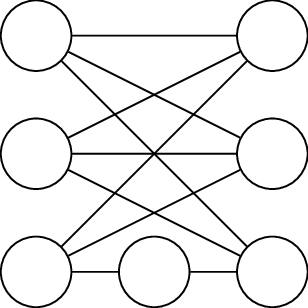
Let the vertices be coloured red and vertices be coloured blue. The path is a Hamiltonian cycle, that we draw as a circle in the plane, as shown below:

This contains 6 of the 9 edges of ; we need to add the edges and . The edge could be drawn inside the circle or outside, suppose we draw it inside, as shown below, with the added edge dashed.
![]()
Then on the inside of the circle, and are on different sides of the line , and so the edge connecting them must go outside the circle. The added edge could go around the right of the circle, as shown below here:

or around the left, as shown here:

But now and are different sides of inside the circle, and on different sides of outside the circle, and so cannot be connected without making two edges cross.
If we had began by drawing outside the circle, then we would have had to draw inside the circle, and had the same problem with being able to draw the last line; as shown here:

An unnecessary case and steoreographic projection
In the proof as presented, we do two cases that seem essentially identical – namely, whether the first edge was drawn inside the circle or outside the circle. In a good proof you don’t want to consider more cases than necessary, so it’s worth stopping to see if these cases are really “the same” or not.
At first glance, the inside and outside of the circle seem to appear very different: the inside has finite area, while the outside has infinite area. However, here’s a slightly different situation where the inside and outside are obviously interchangable: replace with the sphere , and draw the circle as the equator. Then the “inside” is the northern hemisphere, and the “outside” is the southern hemisphere, and obviously we can just do a reflection to interchange them.
It seems like a huge leap to replace the plane with the sphere, but the sphere is really just the plane with one additional point! Put another way, suppose we could draw on the sphere. Our drawing would miss at least point, and if we cut open the sphere at that one point we could stretch the sphere out and lay it flat on the plane, giving a drawing of on the plane.
That sounded vague, but one way it can be made precise is the following: through stereographic projection, which the wikipedia page makes look complicated, but is really just this picture:
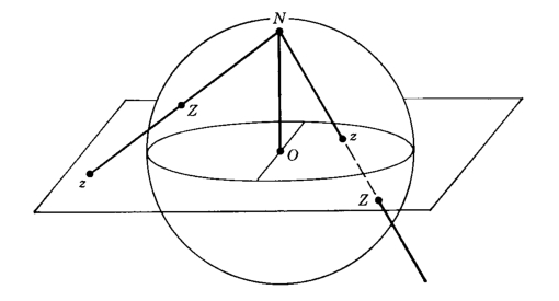
Draw the sphere as the unit sphere centerred at the origin, so the North pole is the point . Then, for any point on the sphere, there is a unique line through and . That line will meet the plane in a unique point . Similarly, given any point in the plane, the line through and will meet the sphere in one other point . This gives a bijection between points on the plane, and points on there sphere (except for the north pole).
If discussion above we slightly lacking, there are lots of fun videos showing (variations of) stereographic projection on youtube. I mentioned in particular Henry Segerman’s videos that illustrated this using shadows and 3-d printed spheres.
Back to planar graphs
If that digression into topology seemed long and pointless, the upshot is that if we’re trying to prove a Hamiltonian graph is nonplanar, we can treat the inside and the outside of the circle as equivalent, and so when we try to add the very first edge we may as well put it inside. This gives us one less choice, and so makes our proofs about half as long! We will use this trick to show that:
The complete graph isn’t planar
The proof is similar, in that we begin by picking a Hamiltonian cycle, say, , and drawing this as a cirlce in the plane, and then try to add the remaining edges. has edges, and 5 are contained in the cycle, so we have 5 more edges to add – and .
Since the inside and outside of the circle are equivalent, we will assume the first edge is drawn inside the circle, giving us the following picture:

It may be tempting to next consider the edge , but this could be drawn either inside or outside the circle, and so we’d have to start considering cases. We get a shorter, cleaner proof if we now move on to the vertex .
The vertex is separated from and on the inside of the circle by the line , and hence the edges and must be drawn on the outside of the circle. These edges separate from on the outside of the circle, and so this must be drawn inside, giving the following picture:

But now we cannot add the final , as and are separated from each other on both the outside and the inside of the circle.
Generalization: The planarity algorithm for Hamiltonian Graphs
The arguments we made to show and aren’t planar can be adapted to easily give a criterion for whether or not any Hamiltonian graph is planar or not.
Suppose is Hamiltonian, and choose a Hamiltonian cycle ; If is planar, then will be drawn as a circle, and every other edge must either lie entirely inside or outside the graph. Now if we pick two edges and that are not part of the cycle, two things can happen depending on the ordering of along the circle:
- If the vertices of and do not interlace (e.g. ), or if they share a vertex (e.g. ); then and may both be drawn inside or outside the circle without crossing.
- If the vertices of and do interlace (e.g. ), then if and are drawn both inside or both outside the circle, they most cross.
So, to see if the whether or not is Hamiltonian, we must look at all the edges that aren’t in , and see if we can split them into two sets, one to be drawn inside, and one to be drawn outside, so that it can be done without crossing. It turns out there’s a slick way to do this.
Definition: Crossing graph
Let be a Hamiltonian graph and and Hamiltonian cycle in . The crossing graph of and , denoted Cross(), has vertices the edges of that aren’t in the cycle, and an edge between two vertices and if the vertices of the corresponding edges interleave, that is, and are adjacent if they cannot be drawn on the same side of the cycle without crossing.
The Planarity Algorithm for Hamiltonian graphs
Suppose is Hamiltonian, with a Hamiltonian cycle. Then is planar if and only if Cross() is bipartite.
Proof:
is bipartite if and only if we can split the edges not in into two sets, inside and outside, so that we can draw each set entirely inside or outside without crossing. But two edges cross if and only if their corresponding vertices in Cross() are adjacent. So trying to draw the edges of without crossing is exactly trying to
Example:
One can check that Cross() will be a three cycle for any choice of Hamiltonian cycle, and Cross() will be a five cycle; neither of which is Hamiltonian.
Example:
Consider the graph shown in the following picture:

It’s obviously Hamiltonian with cycle , and its crossing graph with respect to this cycle is the following:

For example, in the edge crosses the three edges and , and so in Cross(), the vertex is adjacent to those vertices.
It is clear from the picture that Cross() is bipartite, for instance, we may colour and red, and the other three vertices blue. But this tells us how to draw the graph of in the plane – we draw all the red vertices inside the cycle, and the blue vertices outside the cycle, giving the following:

Last session we proved that the graphs and are not planar. We now discuss Kuratowski’s theorem, which states that, in a well defined sense, having a or a are the only obstruction to being non-planar.
We begin with some two simple observations.
Observation 1
If is a subgraph of , and is not planar, then is not planar.
Proof
If we could draw in the plane, it would produce a drawing of in the plane, a contradiction.
As an immediate corrolary, we see that is not planar for , as all such complete graphs contain as a subgraph; similarly, are not planar, with .
Our second observation is the following: suppose we took a graph , and made a new graph by adding one vertex of degree 2 in the middle of one of the edges of . Then drawing is basically the same as drawing , and then sticking an extra dot on an edge. Hence, will be planar if and only if was.
We now make this precise:
Definition
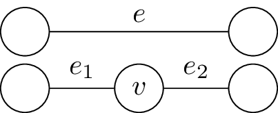
We say that is a subdivision of if it is obtained from by repeatedly choosing an edge and splitting it into two by adding a new vertex, as in the following picture:
Observation 2
Suppose that is a subdivision of . Then is planar if and only if is.
Example
The following graph is nonplanar, since it is obtained from by subdividing a single edge.
Putting together the two lemmas, we see that if has a subgraph , so that is a subdivision of a non-planar graph (like or ), then we isn’t planar. We illustrate this now in an exmaple.
Example: The Petersen graph is not planar
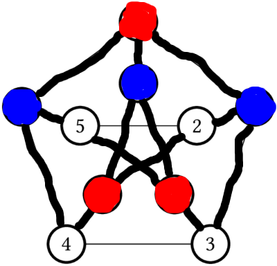
The subgraph drawn with thick edges (containing all but two of the edges in the Petersen graph) is homeorphic to . we have drawn three vertices blue and three vertices red to highlight the vertices of . The nonhighlighted edges are in the subgraph, but they are the ones that are forgetten to show that the highlighted graph is homeomorphic to .
Kuratowski’s Theorem
A graph is nonplanar if and only if it contains a subgraph homeomorphic to or .
Our two observations, together with this morning’s result that and are nonplanar, prove the “if” direction. The “only if” direction is much harder, and we will not prove it.
However, we will only use the “only if” direction implicitly. Using the “only if” direction explicitly would amount to prove that some graph was planar by showing it had no subgraphs that were subdivisions of or , which we would be quite laborious. We have a much easier way to prove that a graph is planar: drawing it in the plane.
We will however, use the “only if” direction implicitly in the following way. Suppose we have a graph , and we want to determine if is planar or not. We can try to prove it is planar by trying to draw it in the plane, and we can try to prove it is not planar by finding a subgraph of that is homeomorphic to either or . The “only if” direction of Kuratowski’s theorem tells us that one or the other of these attempts will always work. Thus, we have a practical method to determine whether or not a graph is planar or not – try to draw it in the plane. If you find this difficult, and begin to expect that it isn’t possible, start looking for a subgraph homeomorphic to either or , which would prove it can’t be drawn on the plane.
Graphs on other surfaces
We now transition to drawing graphs on other surfaces. In lecture, we had some slides providing pictures for the beginning of this discussion; a few, but not all, of those images are in the body of these notes now.
Trying to draw graphs on surfaces can be fun, but it seems like a rather unmotivated question to consider, so we began with motivating it by videogames. Many videogames (pacman, asteroids, overhead RPGs like the early Final Fantasy games) take place on a rectangle screen:
To avoid making the world have an “edge”, the result will often happen: if a character moves off the right of the screen it will reappear at the edge of the left screen, and similarly if a character moves off the top of the screen, it reappears on the corresponding place on the bottom of the screen.
This set-up is used to simulate the surface of a planet. However, if one traces through the result of these identifications, one sees that the surface is a torus:
Definition
A “video-game graph” is one that “locally looks like” a part of graph paper.
Motivating Question
If videogame designers were more clever, could they put a finite videogame graph on the sphere? Can you prove that it isn’t possible?
Drawing graphs on the torus
If we wanted to draw a graph on the sphere, we could do this physically by taking a balloon and a felt pen, but it would be a little awkward to turn in or mark homeworks this way. Luckily, we saw last time that, using stereographic projection, drawing a graph on the sphere is equivalent to being able to draw it on the plane.
Similarly, we could draw graphs on torus by getting donuts, and writing on them with icing sugar. But again, this is rather impractical, and we’d like a way to represent drawing a graph on a torus that is conveniently done on a piece of paper.
The videogame / paper-folding discussion shows us how to do this. We draw a square to represent the torus. On the top and bottom border we draw one arrow in the same direction, to signify that these edges will be identified (this is how the paper was folded, or what a character does in the videogame). We do similar with the side borders, with two arrows.
Then we can draw the graph in the square, with the following added options – if a drawn edge reaches the left (right) border, it continues at the same spot on the right (left) border, and similarly with the top/bottom borders.
Example
and cannot be drawn on the plane, but they can be drawn on the torus as follows:
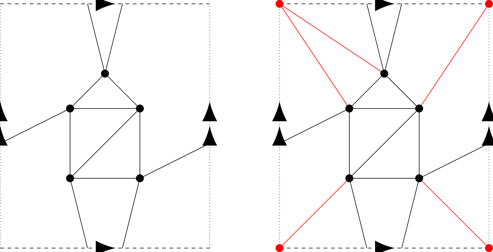
The graph on the left shows on the torus. The picture on the right has the same drawing of in black, but in red has added an extra vertex and 5 extra edges incident to it to make a . There are appear to be 4 red vertices, at each corner of the square, but since all the corners get identified by the folding, they correspond to the same point of the torus.
Challenge
Draw on the torus.
It turns out that cannot be drawn on the torus; we will prove this later.
What comes next?
What other surfaces other than the sphere and torus are possible? One possibility is just adding “more holes”; this produces the “donut with holes”, more formally known as the “suface of genus ”.
You won’t have to work with surfaces of higher genus, but it is worth knowing that this is an active area of research and investigation. It turns out (try to prove it! It’s not hard…) that given any finite graph , there is some so that can be drawn on a surface of genus without the edges crossing. The genus of a graph is defined to be the lowest such that this can be done.
Nonorientable Surfaces
Although you won’t have to work with surfaces of higher genus, you will have to be able to work with a couple of other surfaces. We will end this lecture by introducing the Mobius band:
Unorientable surfaces
In this half of the lecture, we introduce the real projective plane, the simplest closed compact unorientable surface.
Before we do that, it is easiest to review an unorientable surface with boundary that may be more familiar: the Mobius band.
The Mobius band
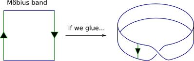
Suppose one has a strip of paper and glues the opposite edges together in the natural way – this makes a cylinder.
If instead, one glued the ends together with half a twist, one would get the Mobius band:
The mobius band is not the same topological space as the cylinder. One way to see this is that it is unorientable – there is not a consistent notion of left and right on the Mobius band. If you start at one point on the Mobius band, and travel along it until you jump across the other side of the identification, you will eventually return to where you started. However, your left and right will have been interchanged! This is seen in the following pictures, stolen from this blog post:
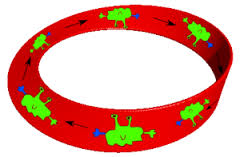
The creature started out, his right hand was blue, but when he returns from his trip around the mobius band it is now his left hand that is blue!
Dual graphs
In the examples at the very beginning of the course, we got a graph from a drawing on the sphere: the Risk board, or more generally, any map.
The countries (or counties or states or whatever region we are working with) are the vertices, and two countries are adjacent if they share a border.
This is different from how we have been thinking about drawing graphs on surfaces – for us, the places where more than two countries meet would be the vertices, and the borders would again be edges. But both of these graphs are coming from the same drawing on the sphere, and so must be related somehow; the concept of dual graphs makes this precise.
Definition
Let be drawn on a surface . The connected components of – i.e., the pieces we would have if we cut along – are called faces
Note: by the Jordan curve theorem, on a sphere, each face will just be a disk. However, this need not be true on a regular surface – for instance, we can get a cylinder as a connected region on the Torus, and the Mobius band as a connected region on the projective plane.
Definition
Let be drawn on a surface , with vertices . The dual graph of is the graph with a vertex for each face of , and an edge for each edge of , that connects the two faces that separates.
It is not hard to see that the faces of the dual graph are the vertices of the original graph, and hence that the dual of the dual graph of is the original graph back.
Euler’s Theorem
Let \(\Gamma\) be a graph drawn on the sphere, and suppose that has vertices, edges, and faces. Then .
Proof idea:
One way to prove it is the following: pick an edge on . If we delete an edge from , we will (usually) merge two faces into one, and thus have one less edge and one less face; this does not change , and gives us a simpler graph where we know by induction.
The only case where deleting the edge doesn’t merge two faces into one is when both sides of the edges are actually the same face; in this case, removing disconnects the graph . One can compute inductively from the two pieces, or perhaps more simply, simply contract the edge in this case, leaving the number of faces unchanged, and reducing the number of edges and vertices by one; again, this doesn’t chave , and will give us a simpler graph where we know by induction.
Applications of Euler characteristic
Euler’s theorem can be very useful in proving results about graphs on the sphere. It’s a bit awkward to use by itself – it contains three variables, and , so it is most useful when we already know some relations between these variables. This may be best illustrated by our motivating example:
Theorem
It is impossible to draw a sphere with a videogame graph.
Proof
Recall that in a videogame graph, every vertex had degree 4, and each face was a square.
Suppose that we had such a graph drawn on the sphere; Euler’s theorem gives us ; we need to use our other knowledge about the graph to get a contradiction.
How can we use that every vertex has degree 4? The handshaking lemma! Since every vertex has degree 4, the sum of the degrees of the vertices is just . So the Handshaking Lemma just says , and hence .
How can we use that every face has four sides? We can do something just like the handshaking lemma, and count the number of times a face meets an edge. On the one hand, each edge meets two faces, and so there are places that an edge meets a face. On the other hand, each face meets four edges, and so we see there are times a face meets an edge, and so we have that , or .
Putting and together, we see that , and so , which is a direct contradiction of Euler’s Formula
It’s worth noting that “handshaking between edges and faces” actually is the handshaking lemma for the dual graph.
To generalize this, we note that we have three sources of relationships between and for a planar graph:
- Euler’s Formula
- Handshaking between vertices and edges
- Handshaking between edges and faces
These three relations can work together to prove a lot. We give one more example now – another proof that and aren’t planar. Yet another example can be found on the last homework set – figuring out how many pentagons a football has.
Application: and aren’t planar
Let’s try to give another proof that and aren’t planar using Euler’s formula.
First, let’s show isn’t planar. We know explicitly that has 5 vertices and 10 edges, so if it were drawn on the sphere we would have
and so it would have to have 7 faces. To get a contradiction, we need another way to get information about how many faces the drawing would have, which we can do via handshaking. has no multiple edges or loops, and so the smallest number of edges a face could have is 3. Thus, handshaking gives us
i.e., . But we know and , so we have a contradiction.
The argument for is similar; we know it has 6 vertices and 9 edges, so if it were drawn on the plane it would need to have 5 faces. is simple, so again we have that each face has at least three sides, but this isn’t strong enough for our purposes. But, since is bipartite, it can’t have any cycles of length three (or any odd number for that matter). Thus, every face of any drawing of must have at least 4 sides. Handshaking between faces and edges then gives , but there are 9 edges and 5 faces, a contradiction.
Application: Footballs have 12 pentagons.
On a football, every vertex is trivalent, but there are two types of faces, pentagons and hexagons. Let be the number of pentagons, and the number of hexagons. Then , so Euler’s theorem gives .
Using handshaking between vertices and edges gives , and using handshaking between faces and edges gives . Thus, we see , where the first equality is vertex-edge handshaking and the second vertex-face. Multiplying Euler’s theorem by 6 gives , and substituting in our deduction from handshaking gives .
Generalization: Euler characteristic and the beginnings of topology
This is more just general mathematical culture than something you would see on the exam.
We have seen for that graphs drawn on the sphere, we have . Given that we’ve discussed drawing graphs on other surfaces, it becomes a natural question to ask if there’s a similar relation for if we have a graph drawn on a different surface . You have to be a little bit more careful in defining what a face is: since the Jordan Curve Theorem fails for surfaces that aren’t the sphere, it is not the case that every component of will be a disk.
However, if we require that is drawn on the surface in such a way so that every “face” is actually a disk, then it turns out that , where is some number, called the Euler characteristic, that depends only on the surface , and not on the graph.
As an example, we saw that video game graphs always had , and the natural way we got to make video game graphs were all living on the torus; the torus has euler characteristic 0.