Section 5.3 Introduction to the chromatic polynomial
For the chromatic number, we were asking whether or not it was possible to colour the vertices of \(\bfG\) with a given number of colours. The chromatic polynomial extends this question, and asks the following. Suppose we have \(k\) colours. How many different ways can we colour the vertices of \(\bfG\text{?}\) It is not clear that this should be a polynomial in \(k\text{,}\) and proving that it is in fact a polynomial in \(k\) is the highlight of the section.
Subsection 5.3.1 Definition and examples
Definition 5.3.1. The chromatic polynomial \(P_{\bfG}\).
The chromatic polynomial \(P_{\bfG}\) of a graph \(\bfG\) is the function that takes in a non-negative integer \(k\) and returns the number of ways to colour the vertices of \(\bfG\) with \(k\) colours so that adjacent vertices have different colours.
It is immediate from the definition of the chromatic polynomial that \(\chi(\bfG)\) is the least positive number \(k\) such that \(\chi_{\bfG}(k)\neq 0\text{.}\)
It is \(not\) immediate from the definition of the chromatic polynomial that it is, in fact, a polynomial. In fact, proving that will take a little bit of work, and we postpone this until the end. First, we look at some examples of the chromatic polynomial; in many cases it is possible to easily compute the chromatic polynomial by working "vertex by vertex".
Example 5.3.2. The empty graph \(E_n\).
Recall that the empty graph \(E_n\) has \(n\) vertices and no edges. To compute \(P_{E_n}(k)\) we need to count the number of ways to colour the vertices with \(k\) colours. But since \(E_n\) has no edges, we can colour each of the \(n\) vertices any of the \(k\) colours; the choices are completely independent. So \(P_{E_n}(k)=k^n\)
Example 5.3.3. The complete graph \(K_n\).
Let's label the vertices \(v_0,\dots, v_{n-1}\text{,}\) and colour them one by one in the given order. When we colour the first vertex \(v_0\text{,}\) no other vertices have been coloured, and we can use whichever of the \(k\) vertice we like. However, when we go to colour \(v_1\) we note that it is adjacent to \(v_0\text{,}\) and so whatever colour we used for \(v_0\) we can't for \(v_1\text{,}\) and so we have \(k-1\) colours to choose for \(v_1\)
Continuing in this way, we see that since all the vertices are adjacent, they all most have different colours. So when we go to colour \(v_i\text{,}\) we have already coloured \(v_o,\dots, v_{i-1}\) with \(i\) different colours, and we can't use any of these to colour \(v_i\text{,}\) and so we have \(k-i\) choices to colour \(v_i\text{.}\)
Putting it all together, we see that:
Example 5.3.4. Two triangles joined at a vertex.
Consider the graph \(\bfG\) consisting of two triangles joined at the right a vertex, shown at the right. We can calulate \(P_\bfG(k)\) by working vertex by vertex: there are \(k\) ways to colour vertex 1, but then when we colour vertex 2 it can't be the same as vertex 1, and so there are \(k-1\) ways to colour it. Vertex three is adjacent to both one and two, so there are \(k-2\) ways to colour it, and vertex 4 is adjacent to one coloured vertex, vertex 3, so there are again \(k-1\) ways to colour it, and finally vertex 5 is adjacent to vertices 3 and 4 and so we have \(k-2\) ways to colour it.Putting it together, we see \(P_\bfG(k)=k(k-1)^2(k-2)^2\text{.}\)

Example 5.3.5. Two triangles joined along an edge.
Consider the graph \(H\) consisting of two triangles joined along an edge. shown at the right. We can calulate \(P_H(k)\) by working vertex by vertex: there are \(k\) ways to colour vertex 1, but then when we colour vertex 2 it can't be the same as vertex 1, and so there are \(k-1\) ways to colour it. Vertex three is adjacent to both one and two, so there are \(k-2\) ways to colour it, and vertex 4 is adjacent to vertices 2 and 3, which have different colours as they are adjacent to each other, so there are \(k-2\) ways to colour it. Putting it together, we see \(P_H(k)=k(k-1)(k-2)^2\)

Subsection 5.3.2 Gluing
What can we say about the chromatic polynomial of a graph \(\bfG\) that's the disjoint union of two smaller graphs: \(\bfG=\bfG_1\sqcup \bfG_2\text{?}\)
We already covered the extreme case where \(\bfG=E_n\) is just a disjoint union of vertices; we could colour each vertex independently of the others, as there were no edges between them at all. A similar argument works in general to give the following.
Proposition 5.3.6.
Let \(\bfG=\bfG_1\sqcup \bfG_2\) be a disconnected graph. Then \(P_{\bfG}(k)=P_{\bfG_1}(k)P_{\bfG_2}(k)\)
Proof.
A colouring of \(\bfG\) with \(k\) colours gives a colouring of \(\bfG_1\) with \(k\) colours and a colouring of \(\bfG_2\) with \(k\) colourings. Similarly, since \(\bfG_1, \bfG_2\) are disconnected, how we colour one will have no effect on what colourings are possible for the other. Hence, colouring \(\bfG\) is exactly the same as colouring \(\bfG_1\) and \(\bfG_2\)
Proposition 5.3.7.
Suppose \(\bfG\) has two subgraphs \(\bfG_1\) and \(\bfG_2\text{,}\) so that their union is all of \(\bfG\text{,}\) but their intersection is a single vertex \(v\text{,}\) i.e. \(\bfG_1\cup\bfG_2=\bfG\) and \(\bfG_1\cap\bfG_2=\{v\}\text{.}\) Then we have the following relation between their chromatic polynomials:
Proof.
As in the proof of colourings of disjoint unions, a colouring of \(\bfG\) gives a colouring of both \(\bfG_1\) and \(\bfG_2\) by restriction, but we don't get any two colourings: both \(\bfG_1\) and \(\bfG_2\) contain \(v\text{,}\) and our two colourings must both make \(v\) the same colouring.
In the other direction, if we have colourings of \(\bfG_1\) and \(\bfG_2\) that have the same colour at \(v\text{,}\) it is clear that we can glue them together to get a colouring of \(\bfG\text{.}\) So the question reduces to the following: given that we want vertex \(v\) to have a fixed colour, how many colourings of \(\bfG_2\) are there that colour \(v\) this colour?
The \(k\) colours are completely interchangeable, however; we could just change the names of each one. Thus, it is clear that there are as many colourings of \(\bfG_2\) where \(v\) is red as there are where \(v\) is blue as there are where \(v\) is any given colour. Hence, if we have \(k\) colours to use, exactly \(1/k\) of all colourings of \(\bfG_2\) will ahve \(v\) any given colour, namely \(P_{\bfG_2}(k)/k\)
Thus, to colour \(\bfG\) with \(k\) colours, we first could first colour \(\bfG_1\) in one of the \(P_{\bfG_1}(k)\) ways. This will give us a some fixed colour of \(v\text{,}\) and we saw above that there are \(P_{\bfG_2}(k)/k\) colourings of \(\bfG_2\) where \(v\) has this colour, and so we have the result.
Example 5.3.8. Two triangles joined at a vertex, again.
As an example, we revisit our previous example. For \(\bfG\text{,}\) two triangles joined at a vertex, we have \(\bfG_1\cong \bfG_2\cong C_3\text{.}\) Since \(C_3\cong K_3\text{,}\) we know \(P_{C_3}(k)=k(k-1)(k-2)\text{.}\) Thus, we have:
Proposition 5.3.9.
Suppose \(\bfG\) has two subgraphs \(\bfG_1\) and \(\bfG_2\text{,}\) so that their union is all of \(\bfG\text{,}\) but their intersection is a single vertex edge \(e\) connecting two vertices \(v\) and \(u\text{,}\) i.e. \(\bfG_1\cup\bfG_2=\bfG\) and \(\bfG_1\cap\bfG_2=\{e\}\text{.}\) Then we have the following relation between their chromatic polynomials:
Proof.
The proof is extremely similar to that of the previous proposition. A colouring of \(\bfG\) gives us colourings of \(\bfG_1\) and \(\bfG_2\text{,}\) but not any two colourings: they need to match at both \(v\) and at \(u\text{.}\)
Now, \(v\) could be any of the \(k\) colours, but \(u\text{,}\) being adjacent to \(v\text{,}\) can't be the same colour, and so it has \(k-1\) possibilities given a choose of colour for \(v\text{.}\) Thus, there are \(k(k-1)\) ways to colour \(v\) and \(u\text{,}\) and all possibilities will occur equally often within the colourings counted by \(P_{\bfG_2}(k)\text{.}\) Hence, given a colouring of \(\bfG_1\text{,}\) there will be \(P_{\bfG_2}(k)/[k(k-1)]\) ways to extendthat colouring to one of all of \(G\text{,}\) giving us the result.
Example 5.3.10. Two triangles joined along an edge, again.
As an example, we revisit our previous example. For \(H\text{,}\) two triangles joined along an edge, we can apply the theorm with \(\bfG_1\cong \bfG_2\cong C_3\text{.}\) Thus, we have:
Subsection 5.3.3 Case by case analysis
The meethods of gluing and working vertex by vertex make many chromatic polynomials easy to calculate. Other graphs, however, are not amenable to our gluing theorems, and require considering several cases when working vertex by vertex.
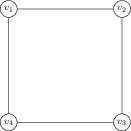
Example 5.3.11. The chromatic polynomial of the cycle \(C_4\).
Now consider the graph \(C_4\text{,}\) shown at right, and suppose we try to count the number of colourings of it with \(k\) colours. Vertex 1 can be any of \(k\) colours, and vertex 2 has \(k-1\) possibilities -- any colour except the one used for vertex 1. Moving to vertex 4, we see it is just adjacent to 1 as well, and so has \(k-1\) possibilities as well.
It becomes more difficult when we try to colour vertex 3. It is adjacent to vertices 2 and 4, and so cannot be the same colour as either of these. However, vertices 2 and 4 are not adjacent, and so we don't know whether they have the same colour or not. If vertices 2 and 4, have the same colour there are \(k-1\) possibilities for vertex 3, while if vertices 2 and 4 have different colours, there are only \(k-2\) possibilties. Thus, we must count how many possibilities are in each of these cases.
If we want vertices 2 and 4 to have the same colour, we can first colour vertex 1 in \(k\) different ways, and then pick any of the remaining \(k-1\) colours for vertices 2 and 4. Then, to complete this to a colouring of \(C_4\text{,}\) we have to colour \(v_3\text{,}\) which can be any of the \(k-1\) colours that aren't the colour \(v_2\) and \(v_4\) are coloured. Thus, the case where \(v_2\) and \(v_4\) have the same colour has \(k(k-1)^2\) possibilities.
If we want vertices 2 and 4 to have different colours, then we can first colour \(v_1\) any of \(k\) colours, colour \(v_2\) any of \(k-1\) colours. Now, when we go to colour vertex 4 it can't be the same colour as vertex 1 since they are adjacent, and it can't be the same colour as vertex 2 by our supposition. Vertices \(v_1\) and \(v_2\) have different colours, and so this leaves \(k-2\) possibilities for \(v_4\text{.}\) Thus there are \(k(k-1)(k-2)\) possibilities to colour vertices 1, 2 and 4 so that 2 and 4 have different colours, and then there are \(k-2\) possibilities left for vertex 3, giving \(k(k-1)(k-2)^2\) ways to colour \(C_4\) so that vertices 2 and 4 have different colours.
Adding the two cases together, this gives:
Example 5.3.12. The chromatic polynomial of \(C_5\).
A similar case-by-case argument that we made for \(C_4\) works for \(C_5\text{,}\) except now we have a further case to deal with. Using the vertex labellings as shown to the right, note that Vertices 3 and 4 must have different colours. We will consider three cases: Vertices 1, 3 and 4 all have different colours, Vertex 1 has the same colour as Vertex 3, and Vertex 1 has the same colour as Vertex 4.

Case 1: 1, 3 and 4 have different colours. Then there are \(k(k-1)(k-2)\) ways to colour vertices 1, 3, and 4, since they must all be different colours. When we go to colour vertices 2 and 5, we see that they are each adjacent to two vertices known to have different colours, and so there are \(k-2\) ways to colour each of them. Thus in total, Case 1 contains \(k(k-1)(k-2)^3\) colourings.
Case 2: 1 and 3 have the same colour. Then there are \(k\) ways to choose this colour, and \(k-1\) ways to choose a colour for vertex 2 (since 1 and 3 have the same colour), and \(k-1\) ways to choose a colour for vertex 4. When we colour vertex 5, we know that 1 and 4 must have different colours, and so we have \(k-2\) ways to colour vertex 5. Thus in total, Case 2 contains \(k(k-1)^2(k-2)\) colourings.
By symmetry, we see that Case 3, where 1 and 4 have the same colour, is identical to Case 2. Thus, putting the three cases together, we see that: