Section 4.2 The planarity algorithm for Hamiltonian graphs
In the previous chapter we showed that \(K_{3,3}\) isn't planar; in this section we investigate how the ideas we used to solve the utilities problem for \(K_{3,3}\)-- namely, the Jordan Curve theorem and the fact that \(K_{3,3}\) is Hamiltonian -- generalize to other graphs. In the end, this will culminate in "The Planarity Algorithm for Hamiltonian Graphs".
Subsection 4.2.1 Stereographic Projection and Unnecessary cases
It will make our life easier if before we investigate other graphs we streamline our proof for \(K_{3,3}\) slightly: there were a few times where we had to treat different cases that wound up behaving essentially the same, and we'd like to see that we didn't actually need to treat them as separate cases. In particular, we would like to show that the following three seemingly different ways to connect the first two vertices lead to the same analysis:
- Connecting them inside the Hamiltonian cycle
- Connecting them outside "to the left"
- Connecting them outside "to the right"

The solution will be to think about drawing the graphs on the sphere \(S^2\) instead of the plane. First, let's see why this solves our problem. On the plane, the inside of a circle is different from the outside of a circle -- the inside is bounded, but the outside is unbounded. However, on the sphere, the two sides of a circle are equivalent -- you can deform any circle to be an equator, and then the northern hemisphere is equivalent to the southern hemisphere. This shows on there sphere, the inside and the outside aren't really different cases.
Furthermore, going around the outside to "the left" or "to the right" are equivalent on the sphere -- you can slowly make the path around the sphere bigger and bigger, and then slip it around the north or south pole, and back. Alternatively, we've already seen that the inside of the circle is equivalent to the outside of the circle on the sphere \(S^2\text{,}\) and on the inside of the circle it doesn't matter exactly how the two points are connected, and so it shouldn't matter on the outside, either.
So we've argued that if we're trying to draw a graph on the sphere, all three cases are the same, but it should still feel like a bait-and-switch: we weren't trying to draw graphs on there sphere, we were trying to draw graphs on the plane. The connection comes from the fact that the sphere can be viewed as a plane with one additional point.
Proposition 4.2.2.
Let \(p\in S^2\) be any point. Then \(S^2\setminus\{p\}\cong\reals^2\text{.}\)Proof.
One way to visualize this is imagine the sphere as being made from very flexible clay. If we poke a small hole in the top of the sphere, we could stick our fingers in and make the hole larger, and gradually stretch and bend and reform for the sphere to be a flat disk, which could be stretched to be the whole plane, in the same way the tangent function maps the interval \((-\pi/2, pi/2)\) to the whole real line \(\reals\)
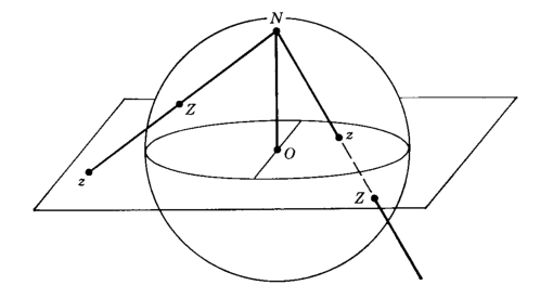
Alternatively, one could use stereographic projection, as shown in Figure . Draw \(S^2\) in \(\reals^3\) as the unit sphere at the origin, and let \(N=(0,0,1)\) be the north pole of the sphere. Stereographic projection gives a bijection between \(S^2\setminus\{N\}\) (the sphere minus the north pole) to the plane, as follows: for any point \(p\neq N\) the line through \(p\) and \(N\) must meet the \(xy\)-plane at one point. On the other hand, any line through \(N\) and a point on the \(xy\)-plane must meet the sphere at one other point.
Accepting that \(S^2\) is \(\reals^2\) minus one point, we see that we can draw a given graph \(\bfG\) on \(S^2\) if and only if we can draw \(\bfG\) on \(\reals^2\text{:}\) if we draw it on \(\reals^2\text{,}\) we can view the \(\reals^2\) as a small patch of \(S^2\text{.}\) And if we have a drawing on \(S^2\text{,}\) there must be at least one point on \(S^2\) that isn't in the drawing of \(G\text{,}\) and doing stereographic projection from that point gives a drawing of \(G\) on the plane \(\reals^2\text{.}\)
Subsection 4.2.2 The planarity algorithm
The preceeding discussion may have felt heavy going, but the upshot is that the cases that seemed "the same" in our analysis of \(K_{3,3}\) actually are the same, and similar cases will be the same for any graph. This will make it much easier to extend our reasoning to more complicated graphs.
Suppose that \(G\) is Hamiltonian, and choose a Hamiltonian cycle; if \(G\) were planar than this cycle must be drawn as a circle, and every other edge must either lie entirely inside or entirely outside the graph. Now consider two edges \(e=ab\) and \(f=xy\) that are not part of the cycle. Depending on the order that \(a,b,x\) and \(y\) appear as you go around the Hamiltonian cycle, one of two things will happen:
- If the vertices of \(e\) and \(f\) do not interlace (e.g. \(abxy, yxab, xbay,\cdots\)), or if they share a vertex (e.g., \(a=x\)), then \(e\) may be drawn both inside or both outside the circle without crossing
- If the vertices of \(e\) and \(f\) do interlace (e.g. \(axby, xayb, yaxb,\dots...\)) then if \(e\) and \(f\) are drawn both inside or both outside the circle, they must cross
This motivates the following definition
Definition 4.2.4. Cross(\(G,C\)).
Let \(G\) be a Hamiltonian graph, and \(C\) a Hamiltonian cycle in \(G\text{.}\) The crossing graph of \(G\) and \(C\text{,}\) denoted Cross(\(G,C\)) has as vertices the edges of \(G\) that aren't in the cycle, and an edge between vertices \(p\) and \(q\) if the vertices of the corresponding edges interleave -- that is, \(p\) and \(q\) are adjacent if they cannot be drawn on the same side of the cycle \(C\) without crossing.
Algorithm 4.2.5. The planarity algorithm for complete graphs.
Suppose that \(G\) is Hamiltonian, and \(C\) is a Hamiltonian cycle. Then \(G\) is planar if and only if Cross(\(G,C\)) is bipartite.
The idea is that if \(G\) is planar, the vertices of Cross(\(G,C\)) are naturally bicolored, with the red vertices, say, corresponding to the edges that are drawn inside the cycle \(C\text{,}\) and the blue edge corresponding to the edges that are drawn outside the cycle \(C\text{.}\) The definition of the edges of Cross(\(G,C\)) guarantees there are no edges between vertices of the same color.
Similarly, if we can find a colouring of the vertices of Cross(\(G,C\)) so that adjacent vertices have different colours, then we can draw all the edges of \(G\) corresponding to red vertices of Cross(\(G,C\)) inside (or outside) \(C\) without having any of them cross.
Example 4.2.6. The complete graph \(K_5\) isn't planar.
Let's apply the planarity algorithm to the complete graph \(K_5\text{.}\) Let's label the vertices 1-5, and take our Hamiltonian cycle \(C\) to be 123451, which we've drawn as the outside pentagon in the following figure: 

Similar consideration with the other edges show that Cross(\(K_5, 123451\)) is the following graph, which is isomorphic to a five cycle:

In particular, Cross(\(K_5, 123451\)) is not bipartite. Hence, by the planarity algorithm for Hamiltonian graphs, we see that \(K_5\) is not planar.
Example 4.2.10. A planar graph.
Let's use the planarity algorithm for Hamiltonian graphs to find a planar drawing of the graph shown in the next figure.

We see that \(H\) is Hamiltonian and take as our Hamiltonian cycle the path around the outside, namely \(abcxyza\text{.}\) There are then six edges not contained in the Hamiltonian cycle, and we find that Cross(\(H, abcxyz\)) is as follows:

For instance, in \(H\) the edge \(ax\) crosses the three edges \(cy, cz\) and \(bz\text{,}\) and so in Cross(\(H, abcxyza\)), the vertex \(ax\) is adjacent to these vertices.
The graph Cross(\(H, abcxyza)\) has no odd cycles and hence is bipartite -- for instance, we may color \(ax, bx\) and \(ay\) red, and the other three vertices blue. Then, to draw \(H\) in the plane without edges crossing, we draw the red edges inside the cycle, and the blue edges outside the cycle:
