Section 3.5 Algorithm for Longest Paths
To complement Dijkstra's algorithm for finding the short path, in this section we give an algorithm for finding the longest path between two vertices in a directed graph.
It is not immediately clear why we might want to do this, so first in Subsection 3.5.1 we give a motivational problem: scheduling work on a complicated project. The algorithm we present will only work on acyclic directed graphs, so in [cross-reference to target(s) "subs_graphalgorithms_longest-path-acyclic-sort" missing or not unique] we define these, explain why this isn't a restriction for our intended application, and give the first step of the algorithm: "topologically sorting" the vertices of an acyclic directed graph. Finally, in Subsection 3.5.2 we explain the actual algorithm.
Subsection 3.5.1
The main application of the longest path algorithm is in scheduling. Suppose we have a large project -- say, building a house -- that is composed of many smaller projects: digging the foundation, building the walls, connecting to gas, electricity, and water, building the roof, doing the interiors, landscaping, etc.
Some of these activities will require others to be done before them (you can't put the roof on before you've built the walls; you don't want to do the landscaping before you've dug your water lines), while others could be done at the same time (finishing the interiors and doing the landscaping). Each sub-job has an expected amount of time required to finish it; you'd like to know before hand how long the whole task will take, and when the various sub-jobs should be done so you can arrange the contractors.
From a series of jobs like this, we will construct a weighted, directed, acyclic graph. The edges will be the sub-jobs. The weights of each edge will be the expected length of time that job has. The structure of the graph will encode the dependencies of the subjobs on each other -- an edge \(e\) will flow into an edge \(f\) if the job \(f\) immediately depends about the job \(e\text{.}\)
We will work out the construction of this graph in one example. It is not always trivial to construct the directed graph from the table of jobs and dependencies. It is not clear what the vertices should be, and sometimes dummy edges and vertices need to be encoded. You do not need to worry about constructing these graphs in general, though if you're curious it can be interesting to think about. Any exam question about this topic would supply you with the directed graph.
Subsubsection 3.5.1.1 Our running example
Consider the following table, listing tasks \(A-H\text{,}\) the expected time of completion for each task, and the required tasks before a given task can be started.
| Task | Time | Prerequisites |
| A | 6 | |
| B | 7 | |
| C | 4 | A |
| D | 3 | A |
| E | 4 | B,D |
| F | 10 | C |
| G | 3 | C |
| H | 10 | E,G |
Here is the corresponding graph encoding this information:
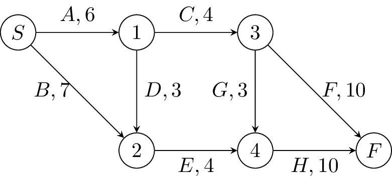
We outline how the graph above was constructed. We make one vertex for the start, one vertex for the finish, and then another vertex for each set of dependencies, that is, the entries in the third column. Then we draw an edge for each letter, beginning at the vertex corresponding to its set of prerequisites (or the start, if it has none), and ending at the vertex that contains it as a prerequisite (or the end, if no tasks require it as a prerequisite).
Note that this method works only if any two sets of prerequisites either have nontrivial intersection or are identical. The tricky cases you don't have to worry about are when this isn't true.
With that detour out of the way, we see why finding the longest path in a directed acyclic graph is useful: in case the edges are tasks and the weights are expected times, the length of the longest path is the minimal time the whole project would be able to be completed.
Moreover, it is useful to actually know what the longest paths are -- to achieve this minimal time, each task in the longest path must be completed in the expected amount of time, and the next task in the path must be started immediately when the first one finishes. For this reason, the longest paths are known as critical paths.
Subsection 3.5.2 Longest Path Algorithm
We now describe an algorithm for finding the longest paths from a starting vertex \(S\) to all other vertices. In some ways, it is similar to Dijkstra's algorithm, in that we will keep a list of "tentative longest paths found so far", and iteratively mark one of these to a vertex \(v\) as an actual longest path, and then update our list with potentially new longest paths by combining our longest path to \(v\) with the edges out of \(v\text{.}\) The main difference is that the ordering this updating will happen will be chosen at the beginning -- any ordering of the vertices compatible with the directed graph structure will work. These orderings are sometimes known as a "topological sort".
Subsubsection 3.5.2.1 Topolgical sort
The first step of the Longest Path Algortihm is to number/list the vertices of the graph so that all edges flow from a lower vertex to a higher vertex. Such a listing is known as a "compatible total ordering" of the vertices, or a "topological sort" of the vertices. For such a list to exist, it is necessary for the graph to be acyclic. Otherwise, we get a "what came first, the chicken or the egg?" type situation. For instance, if we had a directed cycle \(A\to B\to C\to A\text{,}\) we couldn't choose any of \(A, B,C\) to put first, as each one has an error into it from the other vertices.
In our running example graph, the vertices are already numbered in a way compatible with the edge structure, and so is already topologically sorted: \(S,1,2,3,4,F\) is an ordering satisfying the desired properties.
It turns out that this is the only obstacle, and as long as the graph is acyclic, it will have a compatible total ordering. It is not too hard to prove this carefully using induction, and to turn the proof into a constructive algorithm into how to do it, and we invite you to do so. However, in practice for small graphs it is usually not hard to find total orderings. Start with a source (a vertex with no incoming edges, only outgoing edges), then continually look for vertices that only have incoming edges from vertices already on our list.
Finally, we should stress that the topological sort of the vertices is usually not unique. For instance, in our running example, there is no edge between 2 and 3, so instead of \(S,1,2,3,4,F\) we could have ordered the vertices as \(S,1,3,2,4,F\text{,}\) and it also would have been a total ordering. It won't matter which total ordering you choose -- the longest path algorithm will still work. In practice applications a valid total ordering will often be 'obvious'.
Subsubsection 3.5.2.2 The Algorithm
Having topologically sorted the vertices, we find the longest path to each other vertex inductively, by ordering of their numbers. Suppose that we have found the longest paths to each vertex with number lower than \(k\text{,}\) and we want to find the length of the longest path to vertex \(k\text{,}\) which we will call \(u\text{.}\)
Let \(e_i\) be the edges that come into \(u\text{,}\) let \(w(e_i)\) be the lengths of these edges, and let \(v_i\) be the source vertex of \(e_i\text{.}\) Since our edges go from lower numbered vertices to higher numbered vertices, all the \(v_i\) are labelled with numbers lower than \(w\) (i.e., lower than \(k\)), and hence by the inductive hypothesis we know the longest paths to \(v_i\text{.}\) Let \(\ell(v_i)\) be the length of this longest path from \(S\) to \(v_i\text{.}\)
Any path to \(w\) must pass through one of the \(v_i\text{,}\) and so the length of the longest path to \(u\) is the
Typically we will want to find the longest path in addition to just knowing its length, and an easy way to do this is to record the edges \(e_i\) that achieve the maximum. Then we can find the long paths in reverse by starting from \(F\) and going to any recorded vertex.
Example 3.5.2.
We illustrate the longest path algorithm with our example graph. Our start vertex is \(S\text{,}\) and so \(\ell(S)=0\text{.}\)
Vertex 1 has only one incoming edge: \(A\text{,}\) with weight 6, and so \(\ell(1)=6+\ell(S)=6\text{.}\)
Vertex 2 has two incoming edges: \(B\) and \(D\text{,}\) and so we see that \(\ell(2)\) is the maximum of \(w(D)+\ell(1)=3+6=9\text{,}\) and \(w(B)+\ell(S)=7+0=7\text{,}\) and so \(\ell(2)=9\text{.}\)
Vertex 3 has just one incoming edge: \(C\text{,}\) and so \(\ell(3)=w(C)+\ell(1)=4+6=10\text{.}\)
Vertex 4 has two incoming edges: \(G\) and \(E\text{,}\) and so \(\ell(4)\) is the maximum of \(w(G)+\ell(3)=3+10=13\) and \(w(E)+\ell(2)=4+9=13\text{.}\) Thus, the maximum is achieved in two different ways, and we see that there are two paths of length 13 from \(S\) to \(4\) -- \(S-1-3-4\) and \(S-1-2-4\text{.}\)
Finally, vertex \(F\) has two incoming edges, \(F\) and \(H\text{,}\) and so \(\ell(F)\) is the maximum of \(w(F)+\ell(3)=10+10=20\) and \(w(H)+\ell(4)=10+13=23\text{.}\) There are two paths that achieve this maximum -- \(A-C-G-H\) and \(A-D-E-H\text{.}\)
Subsubsection 3.5.2.3 Critical path analysis
Apart from knowing the minimum time for completion of the project, finding the longest paths is useful for analysing where to put resources. In particular, which tasks, if they run slightly over, would make the whole project run late? Which tasks, if they were able to finish slightly early, would make the whole project finish early?
To make the whole project run later, we need to increase the length of the longest path, which means we to increase the length of *any* long path. Thus, the edges that would make the whole project run over are those contained in *any* longest path -- in our graph, these are edges \(A,C,D,E, G\) and \(H\text{.}\)
To make the whole project finish early, we need to decrease the length of *every* longest path, and so these are the edges that are included in *every* longest path. In our graph, these are edges \(A\) and \(H\text{.}\)
These ideas can be developed further, to list for each task the earliest possible starting time, and the latest starting time that is possible while still finishing the whole project in the minimum amount of time.