Section 2.3 Hamiltonian cycles
We now introduce the concept of Hamiltonian walks. Though on the surface the question seems very similar to determining whether or not a graph is Eulerian, it turns out to be much more difficult.
Definition 2.3.1.
A graph is Hamiltonian if it has a closed walk that uses every vertex exactly once; such a path is called a Hamiltonian cycle
First, some very basic examples:
- The cycle graph \(C_n\) is Hamiltonian.
- Any graph obtained from \(C_n\) by adding edges is Hamiltonian
- The path graph \(P_n\) is not Hamiltonian.
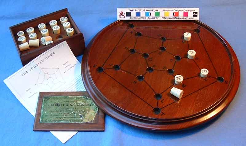
The term Hamiltonian comes from William Hamiltonian, who invented (a not very successful) board game he termed the "icosian game", which was about finding Hamiltonian cycles on the dodecahedron graph (and possibly its subgraphs).
The main thing you'll need to be able to do with Hamiltonian graphs is decide whether a given graph is Hamiltonian or not. Although the definition of Hamiltonian graph is very similar to that of Eulerian graph, it turns out the two concepts behave very differently. While Euler's Theorem gave us a very easy criterion to check to see whether or not a graph Eulerian, there is no such criterion to see if a graph is Hamiltonian or not. It turns out that deciding whether or not a graph is Hamiltonian is NP-complete, meaning that if we could solve that problem efficiently, then you could solve a host of other difficult problems efficiently as well.
It may seem unfair, then, to ask whether a graph is Hamiltonian or not. But it's only in a very theoretical way that the problem is extremely difficult -- as the number of vertices get very large, the problem gets harder and harderquickly. For any given graph with a low number of vertices, there aren't that many possibilities to check.
If a graph is Hamiltonian, then by far the best way to show it is to exhibit a Hamiltonian cycle, as in Figure 2.3.2. When the graph isn't Hamiltonian, things become more interesting.
The most natural way to prove a graph isn't Hamiltonian is to do a case by case analysis of possible paths, showing it doesn't work. For instance, in lecture we outlined the proof that if you remove a vertex from the Icosian graph, than the result isn't Hamiltonian. A natural way to do this is to pick a vertex, and consider the possible pairs of edges the path might take through that vertex. For each possibility, we know some edges won't be used, and can go further along that way.
In general, brute-force case-by-case analyses are proofs we want to avoid when possible, because it can be difficult to make sure we have actually found all the cases, and the proofs aren't always enlightening. It's much better when we can find a "reason" why the graph isn't Hamiltonian.
Example 2.3.3.

Figure 2.3.4 shows a portion of a larger graph \(\bfG\text{.}\) The exact number of other vertices in the graph that \(X\) and \(Y\) are adjacent to is not important; what matters is that \(A\) and \(B\) are each adjacent to two vertices, \(X\) and \(Y\text{.}\) Any path through \(A\) would have to use \(X\) and \(Y\text{,}\) but so would any path through \(B\text{.}\) But then we have a small four cycle \(XAYBX\) which doesn't use any other vertices in the graph, and so \(\bfG\) cannot be HAmiltonian.
Lemma 2.3.5.
Suppose that \(\bfG\) is bipartite and Hamiltonian, with \(n\) red vertices and \(m\) blue vertices.
Proof.
Consider a Hamiltonian path in \(\bfG\text{.}\) Since every edge is between a red and blue vertex, the vertices in the path must alternate between red and blue. Considering every other edge of the cycle pairs each red vertex with a blue vertex, and hence \(n=m\text{.}\)
The contrapositive of Lemma 2.3.5 can be used to show graphs aren't Hamiltonian: if \(\bfG\) is bipartite but doesn't have the same number of red vertices and blue vertices, then it can't be Hamiltonian.
Lemma 2.3.6.
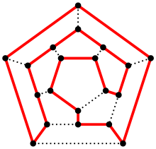
The Petersen Graph is not Hamiltonian
Proof.
Of course, a case-by-case analysis of possibile Hamiltonian cycles is possible. The number of cases can be reduced by using symmetries of the Petersen graph. Instead, for variation and to illustrate a different proof technique, we will use another method.
Assume for contradiction that the Petersen graph is Hamiltonian, and draw the ten vertices \(v_1,v_2,\dots,v_{10}\) around the cycle. The Hamiltonian cycle uses 10 of the 15 edges in the Petersen graph, and so there must be 5 more edges, with each vertex incident to one of them, as in the Petersen graph every vertex has degree 3.
Let's analyse where else the edge adjacent to \(v_1\) could go. It can't go to \(v_1\) itself, as the Petersen graph has no loops, and it can't go to \(v_2\) or \(v_{10}\) as the Petersen graph has no multiple edges. If it went to \(v_3\) or \(v_9\) it would make a three cycle, which the Petersen graph doesn't have, and if it went to \(v_4\) or \(v_7\text{,}\) there'd be a four cycle. Hence, the only options are \(v_1\) is adjacent to \(v_5, v_6\) or \(v_7\text{.}\) By reversing the direction of the Hamiltonian path, \(v_5\) and \(v_7\) are equivalent, and there are only two cases.
But the same analysis holds for every vertex: the extra edge at any vertex can either go to the opposite side of the circle, or be "off by one" and skip three vertices to either direction.
We now claim that not all the extra edges can go "directly across" -- there must be at least one edge that's off by one. If all the extra edges went directly across, then \(v_1\) would go to \(v_6\text{,}\) and \(v_2\) would go to \(v_7\text{,}\) and \(v_1-v_6-v_7-v_2-v_1\) would be a 4 cycle.
Hence, without loss of generality we may assume that the extra edge at \(v_1\) is \(v_1-v_5\text{.}\) Let us then consider the extra edge at \(v_6\text{.}\) It can't go directly across, as that is \(v_1\) which already has its extra edge. Hence it must be off by one, and go to either \(v_2\) or \(v_{10}\text{.}\) But either way we get a four cycle: either \(v_1-v_2-v_6-v_5-v_1\text{,}\) or \(v_1-v_{10}-v_6-v_5-v_1\text{.}\) Hence, we have a contradiction, and the Petersen graph cannot be Hamiltonian.
Finally, Ore's Theorem, a positive result, giving conditions which guarantee that a graph has a Hamiltonian cycle. First, a little bit of intuition. If we take an edge to a Hamiltonian graph the result is still Hamiltonian, and the complete graphs \(K_n\) are Hamiltonian. Thus, one might expect that a graph with "enough" edges is Hamiltonian.
The trick is in finding an interesting meaning of the word "enough". Simply counting the number of edges does not give very interesting bounds on what "enough" means, however -- the complete graph has \(n(n-1)/2\) edges, but we can make it non-Hamiltonian by removing only \(n-2\) edges: simply pick a vertex \(v\) and remove all but one of the \(n-1\) edges coming out of \(v\text{;}\) then \(v\) will now have degree 1, and hence the resulting graph cannot be Hamiltonian.
Theorem 2.3.7. Ore's Theorem.
Let \(\bfG\) be a simple graph with \(n\) vertices, and assume that whenever two distinct vertices \(v,w\) are not adjacent, we have \(d(v)+d(w)\geq n\text{.}\) Then \(\bfG\) is Hamiltonian.
Proof.
We will argue by contradiction, and begin by passing to a maximal counterexample. Note that if \(\bfG\) satisfies the hypotheses, and we add an edge \(e\) to \(\bfG\) between two non-adjacent vertices \(v\) and \(w\text{,}\) then the result will still satisfy the hypothesis. Indeed, we've only increased the degree of some vertices. So, we had a counterexample \(\bfG\) to Ore's Theorem, we could iteratively add edges to \(\bfG\) that didn't create Hamiltonian cycles, until we got a graph \(\bfG\) that satisfies the hypotheses of Ore's theorem, desn't have any Hamiltonian cycles, but if we add any edge \(e\) to \(\bfG\) the result is Hamiltonian.
We now observe that such a \(\bfG\) must have a Hamiltonian path: indeed, pick any edge \(e\) not in \(\bfG\) and add it to \(\bfG\text{.}\) THe resulting graph is by assumption Hamiltonian, and since \(\bfG\) wasn't Hamiltonian, the Hamiltonian cycle must contain the edge \(e\text{.}\) Deleting the edge \(e\) from the Hamiltonian cycle gives a Hamiltonian path in \(\bfG\text{.}\)
Thus, let \(v_1-v_2-\cdots v_n\) be a Hamiltonian path in \(\bfG\text{.}\) We know \(v_1\) and \(v_n\) are not adjacent, as otherwise \(\bfG\) would be Hamiltonian. Thus, since \(\bfG\) satisfies the hypothesis of Ore's theorem, we know \(d(v_1)+d(v_n)\geq n\text{.}\) We already have one edge adjacent to \(v_1\text{,}\) and one edge adjacent to \(v_n\text{,}\) and so there must be at least \(n-2\) other edges adjacent to one or other of these vertices. We will see that no matter how we add \(n-2\) edges to these two vertices, we will create a Hamiltonian cycle.
To see this, note there is ever an \(i\) with \(v_1\) adjacent to \(v_i\) and \(v_{i-1}\) adjacent to \(v_n\text{,}\) then \(\bfG\) would have a Hamiltonian cycle: namely \(v_1-v_2-\cdots-v_{i-1}-v_n-v_{n-1}-\vdots v_i-v_1\text{.}\) Now, there are \(n-3\) different vertices we can add edges to \(v_1\) to, namely \(v_3-v_{n-1}\text{,}\) and similarly there are \(n-3\) vertices we can add edges connecting \(v_n\) to, namely \(v_2, \dots v_{n-2}\text{.}\) We arrange these \(2(n-3)\) edges into a a grid with 2 rows and \(n-3\) columns, so that the two edges in each column are \(v_1-v_i\) and \(v_n-v_{i-1}\text{,}\) a pair of edges that can form a Hamiltonian cycle as in the last paragraph.
As we need to add at least \(n-2\) edges, but we only have \(n-3\) columns, there must be at least one column that contains two edges by the pigeonhole principle, but then we can create a Hamiltonian cycle using those two edges and the edges in our Hamiltonian path.
Note that Ore's Theorem is not an if and only if, and so Ore's Theorem cannot be used to prove that graphs aren't Hamiltonian. Indeed, there are plenty of graphs that are Hamiltonian but do not satisfy the hypotheses of Ore's Theorem. For instance, the cycle graph \(C_n\) is Hamiltonian, but every vertex has degree 2, so if \(n\geq 5\) the hypotheses of Ore's Theorem are not satisfied.
We also highlight that the proof began by considering a maximal counterexample to Ore's Theorem, and considering maximal/minimal counterexamples is often a useful proof technique, as you the maximality/minimality gives you some extra structure to work with.