Section 1.5 Trees
A very important class of graphs are trees -- they are connected, but just barely: removing any edge causes them not to be connected.
Subsection 1.5.1 Basics on trees
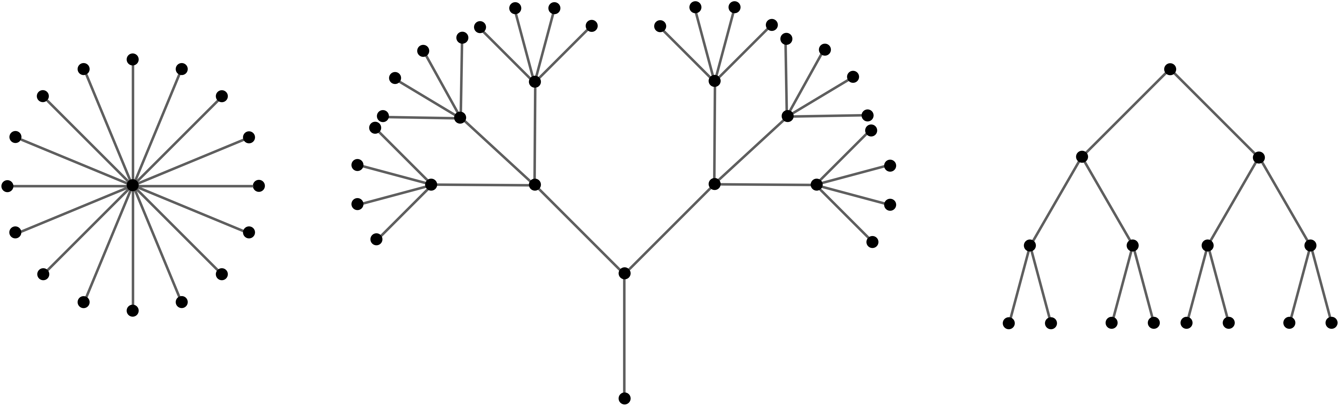
The figure above shows some examples of the trees. Meanwhile, the cycle graph \(\bfC_n\) or the complete graph \(\bfK_n\) with \(n\geq 3\) are not trees: we can remove an edge from these graphs and they'd still be connected. The formal definition of a tree is as follows:
Definition 1.5.2. Trees and Forests.
A graph \(\bfG\) is a tree if:
- \(\bfG\) is connected
- \(\bfG\) has no cycles
A not necessarily connected graph with no cycles is called a forest, so that a forest is a union of trees.
Informally, the condition that \(\bfG\) is connected is asking that \(\bfG\) have enough edges, while the condition that \(\bfG\) has no cycles is asking for \(\bfG\) not to have too many edges. Thus, trees are sort of "goldilocks" graphs -- they have enough edges, but not too many -- they're connected, but just barely.
The following Theorem gives many alternate characterisations of trees, and makes more precise the intuition of trees as "goldilocks graphs"
.Theorem 1.5.3.
Let \(\bfG\) be a graph with \(n\) vertices. The following are equivalent:
- \(\bfG\) is a tree.
- Between any two vertices \(a,b\in V(\bfG)\text{,}\) there is a unique path.
- \(\bfG\) is connected, but removing any edge makes \(\bfG\) disconnected.
- \(\bfG\) has no cycles, but adding any edges to \(\bfG\) creates a cycle.
- \(\bfG\) is connected and has \(n-1\) edges
- \(\bfG\) has no cycles and has \(n-1\) edges
We will not use most of , and will not prove that all options are equivalence. We briefly proof that 1 is equivalent to 2 now, and in the next section we will carefully prove that 1 is equivalent to 5, as we will use this fact a few times. The rest make a good exercise to check your basic understanding.
To see that 1 and 2 are equivalent, note that being connected by definition means there is a path between every two vertices. As a tree is a connected graph without any cycles, to finish seeing 1 and 2 are equivalent is exactly Lemma 1.5.5, whose main idea is contained in Figure 1.5.4

Lemma 1.5.5.
A graph \(\bfG\) has no cycles if and only if there is at most one path between any two vertices of \(\bfG\text{.}\)
Proof.
If \(\bfG\) has a cycle, the there are at least two paths between any vertex on that cycle -- the paths going each way around the cycle. Thus, we just have to show that if there there are two paths between between \(v\) and \(w\text{,}\) then \(\bfG\) has a cycle.
In the easy case, the two paths will contain no vertices in common except for \(v\) and \(w\text{,}\) and so the union of the two paths will be a cycle. In general, the paths will share other vertices and edges -- they may well repeat vertices and edges themselves. But in any case, by considering some subset of these two paths will be a cycle.
Subsection 1.5.2 Leaves
To prove Theorem , we first need to introduce the concept of leaves.
Definition 1.5.6. Leaf.
A vertex \(v\in\bfG\) is called a leaf if it has degree one, i.e. if \(d(v)=1\)
When looked at a drawn graph, this definition is fairly intuitive: real life trees branch out and split in leaves, just like mathematical trees.
Lemma 1.5.7. Trees have leaves.
Let \(\bfT\) be a finite tree with at least two vertices. Then \(\bfT\) has at least two leaves.Proof.
By assumption, \(\bfT\) has at least two vertices, say \(v_0\) and \(w_0\text{.}\) Since \(\bfT\) is a tree it is connected, and so in particular there must be a path between \(v_0\) and \(w_0\text{;}\) let \(v_i\) be the vertices in this path, and let \(e_i\) be the edge in the path joining \(v_{i-1}\) to \(v_i\text{.}\)
Since \(v_m\) is adjacent to \(e_m\) it has degree at least one; if it has degree 1 it is a leaf, and we've found a leaf. If \(v_m\) is not a leaf, then there must be another edge coming out of it, say \(e_{m+1}\) going to \(v_{m+1}\text{.}\) Note that \(v_{m+1}\) cannot be any of the vertices we've already found, as then we'd have more than one path between two vertices and hence a loop, but \(\bfT\) was a tree. Thus we can make the path a bit longer.
We can now continue this argument inductively as long as the vertex at the of the path has degree higher than 1. But since \(\bfT\) is finite, and we never return to a vertex we've already visited, we this process must eventually terminate, but the only way this can happen is if the end vertex of the path has degree 1, that is, if it's a leaf.
A similar argument extending from \(v_0\text{,}\) the other end of the path, shows that we must eventually reach a different leaf from that end, and so \(\bfT\) must have at least two leaves, as desired.
Lemma 1.5.8.
A simple graph \(\bfG\) with \(n\) vertices is a tree if and only if is connected and has \(n-1\) edges.
Proof.
Since being connected is half of the requirement of being a tree, we need to show that a connected graph on \(n\) vertices is a tree if and only if it has \(n-1\) edges.
Let us first prove that a tree on \(n\) vertices has \(n-1\) edges. We will use induction on \(n\text{.}\) As bases, there is only one tree with 1 vertex, and it does in fact have 0 edges, and there is only one tree with two vertices, and it does in fact have 1 edge. So for the inductive step, let us suppose that we know that all trees with \(k\lt n\) vertices have \(k-1\) edges, and let \(\bfT\) be a tree with \(n\) vertices. By Lemma, we know that \(\bfT\) has a leaf \(v\text{,}\) which by the definition of leaves is connected to the rest of \(\bfT\) by a single edge \(e\text{.}\) If we delete \(v\) and \(e\) from \(\bfT\text{,}\) we get a smaller graph \(\bfT^\prime\) ince which has one less vertex and one less edge than \(\bfT\) did.
Since \(\bfT\) was a tree, it follows that \(\bfT^\prime\) is a tree, too -- check this yourself, using the definition of a tree! Then, since \(\bfT^\prime\) is a tree with \(n-1\) vertices, byt the inductive hypothesis it follows that it has one less edge \(n-2\) edges, and so \(\bfT\) must have \(n-1\) edges, which is what we were trying to show.
Now we show the other direction: that if \(\bfG\) is a simple connected graph with \(n\) vertices and \(n-1\) edges, then \(\bfG\) is a tree. The basic structure of the proof is the same as the other direction: find a vertex \(v\) adjacent to a single edge \(e\text{,}\) and delete \(v\) and \(e\) to get a smaller tree, where we can assume the proposition holds, and then use induction.
To play the role of the lemma that every tree has a leaf, we will establish the following statement: if \(\bfG\) is a connected graph with \(n\) vertices and \(n-1\) edges, then /p>\(\bfG\) has a vertex of degree 1. Note that since \(\bfG\) is connected, it can't have any vertices of degree 0, and so to prove it has a vertex of degree 1 it is enough to show that it has a vertex of degree strictly less than 2. Thus, for contradiction assume that every vertex \(v\) of \(\bfG\) has degree \(d(v)\geq 2\text{.}\) But then the handshaking lemma would say:
a contradiction, and hence \(\bfG\) must have a vertex of degree 1, as desired.
Subsection 1.5.3 Trees in Chemistry
Our brief study of trees has the following consequence for chemistry: whether or not a molecule is a tree is determined just by its chemical formula, and not how it's put together. Equivalently, if one isomer of a molecule is a tree, then all isomers of the molecule are.
The argument runs as follows. Knowing the chemical formula of a molecule means we know the degree sequence of the corresonding graphs. Molecules are by definition connected graphs, so to be a tree it is enough to show that the graph has one less edge than the number of vertices. But we can compute the number of edges from the degree sequence by using the Handshaking Lemma.
Example 1.5.9. Alkanes are trees.
Any molecule with formula \(C_nH_{2n+2}\) is an alkane. Although in general alkanes can have multiple isomers, every isomer of an Alkane will always be a tree, as we now show.
To show a graph is a tree, it suffices to show that it is connected and that the number of edges is one less than the number of vertices. Since Alkanes are molecules, we know that the graph is connected. Furthermore, \(C_nH_{2n+2}\) has \(n\) carbons adn \(2n+2\) hydrogens, and hence has \(3n+2\) vertices. Thus, it is enough to show that any molecule with formula \(C_nH_{2n+2}\) has \(3n+1\) edges.
To do this, we use the handshaking lemma: \(2e=\sum d(v)\text{.}\) Each of the \(n\) carbons has degree 4, so the carbons contribute \(4n\) to the total degree, and each hydrogen of the \(2n+2\) has degree 1 and so only contributes 1 to the sum of degrees. Hence, twice the number of edges is equal to \(4n+(2n+2)=6n+2\text{,}\) and so there are \(3n+1\) edges, as desired.
As an early application of graph theory, Cayley used these ideas to count the number of isomers of Alkanes (with some mistakes). In general, you can count isomers of any molecule by counting isomorphism classes of graphs with given degree sequences, but it can help organize the search to know, e.g., that they're all trees. To make sure we don't miss or double count any, it's useful to organize the enumeration according to some principle; for Alkanes one way is to organize according to the longest path of carbons, another is to restrict degree sequences to just how the carbons have connected to other carbons.
Example 1.5.10. Counting isomers of \(C_6H_{14}\).
We illustrate these both of these methods. We first illustrate by length of the longest path of carbons.
- Chain length six: Since we've used all carbons then there are no more choices, and there is only one such isomer.
- Chain length five: We need to add one more carbon. We can't add it to either of the end carbons, because then we'd have a path of length 6. We can add it to the central of the two chains, or alternatively to one either side of central -- the last two trees are isomorphic, giving us two possibilities
- Chain length four: We need to add two more carbons. Again, they can't be added to either of the end carbons, or we'd have a longer chain length. Therefore, they most be added to the two central carbons. One case is that we add one carbon to each of the two central carbons. Alternatively, we could add both the carbons to the same "central" carbon reversing the order of the chain is a symmetry that interchanges the two central atoms. We could add each carbon directly to the existing carbon in the chain, or we could add them one after the other making a chain of length two. However, the resulting graph would have a chain of length 5 and already be counted. Thus, there are two possibilities here.
- Chain length three: We need at add three more carbons, and there's only one central carbon to attach them to. We can't add them all directly to this central carbon, as that would create a carbon of degree 5. On the other hand, once we add a chain of length longer than one to this central carbon we'd have a path of length 4 or greater.
Thus, we see there are five isomers of \(C_6H_{14}\text{.}\) Alternatively, we could organize our search by deleting the hydrogens, and then considering the degrees of the resulting carbon-carbon graph.
- Degree at most two: If the resulting tree only had carbons of degree at most two, then it would have to be the path graph \(P_6\text{,}\) and so we only have one possibility here.
- One vertex of degree three: If the resulting graph had exactly one carbon of degree three, that vertex and its three neighbours would account for 4 of our 6 carbons, and so we'd have to add two more. We couldn't add them directly to the same vertex, as that would create a second vertex of degree three. So, they could either be added as a chain of length two to one of the leaves of the existing graph, or they could be added to two separate leaves. Drawing these graphs we see they're not isomorphic, and so we have two possibilities here.
- Two vertices of degree three: If we have two vertices of degree three, one sees they'd have to be adjacent to each other, resulting in one possibity.
- Vertex of degree four: A vertex of degree 4 and its four neighbours would account for all but one of the carbons. We could add that carbon to any of the leaves, and get one more possiblity.

Since carbons only have degree 4, the tree with six vertices where all are connected to a central vertex isn't allowed, and we have found all the isomers.